Advanced Heating and Cooling Settings#
This notebook demonstrates how to control individual heating and cooling mechanisms in UCLCHEM using the HeatingSettings class. We’ll:
Run a baseline model with all mechanisms enabled
Analyze which heating and cooling processes dominate
Disable the most important mechanisms
Compare the results to understand their impact
This is useful for understanding which physical processes drive the thermal evolution in your model.
import os

import matplotlib.pyplot as plt

import uclchem
from uclchem import advanced

# Ensure output directory exists
os.makedirs("../examples/test-output", exist_ok=True)
Step 1: Run Baseline Model with All Mechanisms#
First, let’s run a standard cloud model with all heating and cooling mechanisms enabled and retrieve detailed rate information.
# Define model parameters for a molecular cloud
param_dict = {
    "initialDens": 1e4,  # Initial density (cm^-3)
    "initialTemp": 10.0,  # Initial temperature (K)
    "finalTime": 1.0e6,  # Final time (years)
    "baseAv": 10.0,  # Visual extinction
    "rout": 0.1,  # Outer radius (pc)
    "freefall": False,  # Keep constant density
    "heatingFlag": True,  # Enable heating (default)
}

# Run the baseline model with all mechanisms enabled
print("Running baseline model with all heating/cooling mechanisms enabled...")
cloud_full = uclchem.model.Cloud(param_dict=param_dict)

# Extract all data from the model object in one call
physics_full, abundances_full, rate_constants_full, heating_full = cloud_full.get_dataframes(
    joined=False, with_rate_constants=True, with_heating=True
)
start_abund = cloud_full.next_starting_chemistry_array
flag_full = 0 if cloud_full.has_attr("_data") else -1

print(f"Baseline model completed with flag: {flag_full}")
if flag_full == 0:
    print(
        f"Temperature range: {physics_full['gasTemp'].min():.2f} - {physics_full['gasTemp'].max():.2f} K"
    )
    print(f"Final temperature: {physics_full['gasTemp'].iloc[-1]:.2f} K")
else:
    print("Error: Model failed to complete")
Running baseline model with all heating/cooling mechanisms enabled...
Baseline model completed with flag: -1
Error: Model failed to complete
Step 2: Identify the Most Important Heating and Cooling Processes#
Let’s analyze the heating DataFrame to determine which heating and cooling mechanisms contribute the most.
# Extract heating and cooling columns
heating_cols = [col for col in heating_full.columns if col.endswith("Heating")]
cooling_cols = [col for col in heating_full.columns if col.endswith("Cooling")]

print(f"Found {len(heating_cols)} heating processes")
print(f"Found {len(cooling_cols)} cooling processes")

# Calculate the total integrated contribution of each process over the entire simulation
# Use absolute value to capture magnitude regardless of sign
heating_importance = {}
for col in heating_cols:
    # Sum the absolute values over time to get total contribution
    total_contribution = heating_full[col].abs().sum()
    heating_importance[col] = total_contribution

cooling_importance = {}
for col in cooling_cols:
    total_contribution = heating_full[col].abs().sum()
    cooling_importance[col] = total_contribution

# Sort by importance
heating_sorted = sorted(heating_importance.items(), key=lambda x: x[1], reverse=True)
cooling_sorted = sorted(cooling_importance.items(), key=lambda x: x[1], reverse=True)

# Display top 5 heating processes
print("\n" + "=" * 70)
print("TOP 5 HEATING PROCESSES (by integrated absolute contribution)")
print("=" * 70)
for i, (process, contribution) in enumerate(heating_sorted[:5], 1):
    process_name = process.replace("Heating_", "")
    print(f"{i}. {process_name:40s} {contribution:.2e} erg cm⁻³ s⁻¹ yr")

# Display top 5 cooling processes
print("\n" + "=" * 70)
print("TOP 5 COOLING PROCESSES (by integrated absolute contribution)")
print("=" * 70)
for i, (process, contribution) in enumerate(cooling_sorted[:5], 1):
    process_name = process.replace("Cooling_", "").replace("LineCooling_", "")
    print(f"{i}. {process_name:40s} {contribution:.2e} erg cm⁻³ s⁻¹ yr")

# Store the most important ones for later
top_heating_process = heating_sorted[0][0] if heating_sorted else None
top_cooling_process = cooling_sorted[0][0] if cooling_sorted else None

print(f"\nMost important heating: {top_heating_process}")
print(f"Most important cooling: {top_cooling_process}")
Found 10 heating processes
Found 12 cooling processes
======================================================================
TOP 5 HEATING PROCESSES (by integrated absolute contribution)
======================================================================
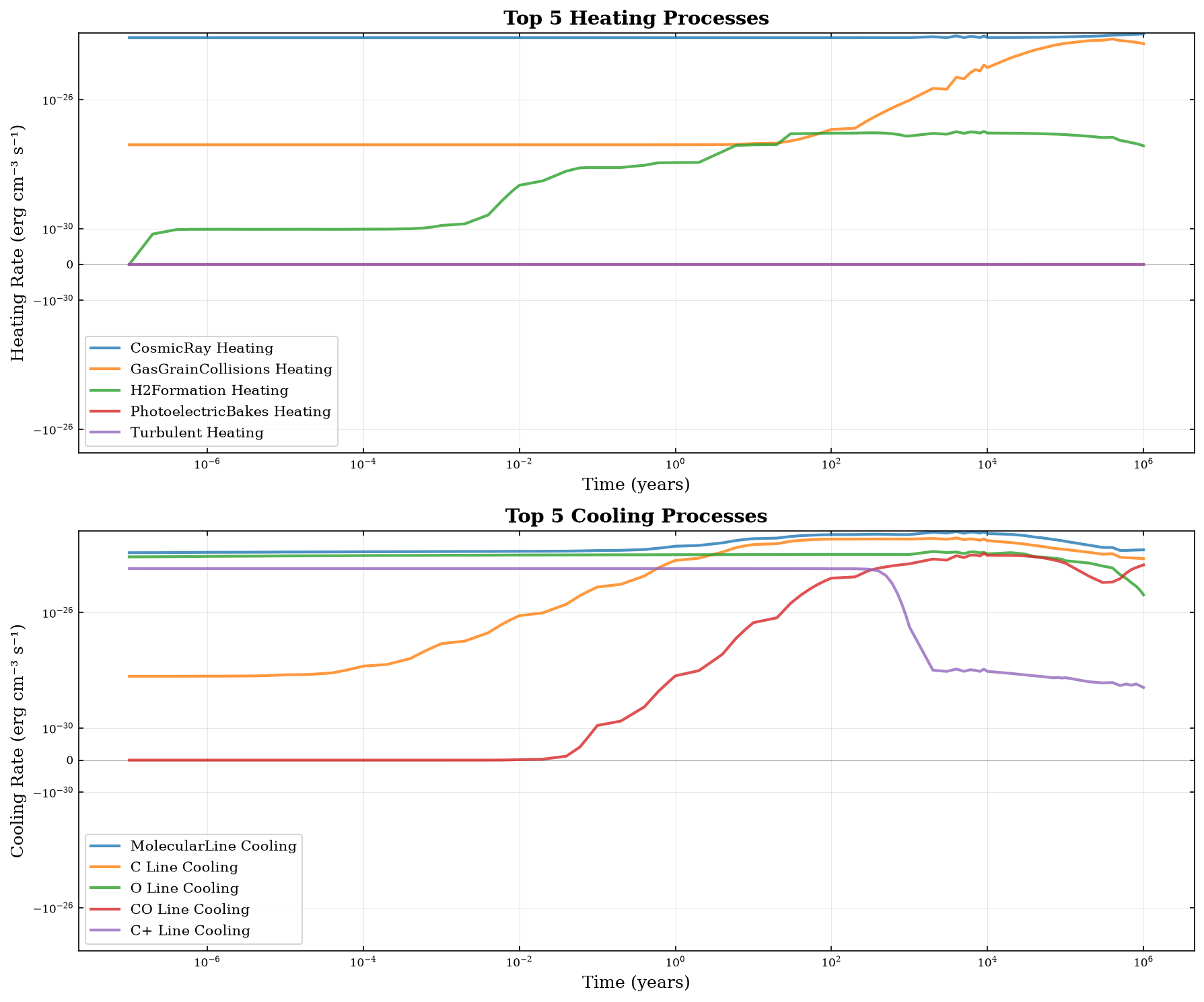
1. CosmicRay Heating 7.42e-23 erg cm⁻³ s⁻¹ yr
2. GasGrainCollisions Heating 1.02e-23 erg cm⁻³ s⁻¹ yr
3. H2Formation Heating 3.88e-26 erg cm⁻³ s⁻¹ yr
4. PhotoelectricBakes Heating 7.59e-33 erg cm⁻³ s⁻¹ yr
5. Turbulent Heating 6.06e-38 erg cm⁻³ s⁻¹ yr
======================================================================
TOP 5 COOLING PROCESSES (by integrated absolute contribution)
======================================================================
1. MolecularLine Cooling 2.50e-22 erg cm⁻³ s⁻¹ yr
2. C Line Cooling 1.26e-22 erg cm⁻³ s⁻¹ yr
3. O Line Cooling 7.75e-23 erg cm⁻³ s⁻¹ yr
4. CO Line Cooling 2.10e-23 erg cm⁻³ s⁻¹ yr
5. C+ Line Cooling 1.78e-23 erg cm⁻³ s⁻¹ yr
Most important heating: CosmicRay Heating
Most important cooling: MolecularLine Cooling
Step 3: Visualize the Dominant Processes#
Let’s plot the time evolution of the most important heating and cooling processes.
fig, axes = plt.subplots(2, 1, figsize=(12, 10))

time = heating_full["Time"]

# Plot top 5 heating processes
axes[0].axhline(y=0, color="k", linestyle="-", linewidth=0.5, alpha=0.3)
for process, _ in heating_sorted[:5]:
    label = process.replace("Heating_", "")
    axes[0].plot(time, heating_full[process], label=label, linewidth=2, alpha=0.8)

axes[0].set_xlabel("Time (years)", fontsize=12)
axes[0].set_ylabel("Heating Rate (erg cm⁻³ s⁻¹)", fontsize=12)
axes[0].set_xscale("log")
axes[0].set_yscale("symlog", linthresh=1e-30)
axes[0].set_title("Top 5 Heating Processes", fontsize=14, fontweight="bold")
axes[0].legend(fontsize=10, loc="best")
axes[0].grid(True, alpha=0.3)

# Plot top 5 cooling processes
axes[1].axhline(y=0, color="k", linestyle="-", linewidth=0.5, alpha=0.3)
for process, _ in cooling_sorted[:5]:
    label = process.replace("Cooling_", "").replace("LineCooling_", "")
    axes[1].plot(time, heating_full[process], label=label, linewidth=2, alpha=0.8)

axes[1].set_xlabel("Time (years)", fontsize=12)
axes[1].set_ylabel("Cooling Rate (erg cm⁻³ s⁻¹)", fontsize=12)
axes[1].set_xscale("log")
axes[1].set_yscale("symlog", linthresh=1e-30)
axes[1].set_title("Top 5 Cooling Processes", fontsize=14, fontweight="bold")
axes[1].legend(fontsize=10, loc="best")
axes[1].grid(True, alpha=0.3)

plt.tight_layout()
plt.show()
/tmp/ipykernel_3713/4153037787.py:33: UserWarning: The figure layout has changed to tight
  plt.tight_layout()
Step 4: Introduction to HeatingSettings#
The HeatingSettings class allows you to control individual heating and cooling mechanisms. Let’s explore what’s available.
# Create a HeatingSettings instance
settings = advanced.HeatingSettings()

# Get all available heating mechanisms
heating_mechanisms = settings.get_heating_modules()
cooling_mechanisms = settings.get_cooling_modules()

print("AVAILABLE HEATING MECHANISMS:")
print("=" * 70)
for mech, active in heating_mechanisms.items():
    status = "✓ ACTIVE" if active else "✗ INACTIVE"
    print(f"  {mech:40s} {status}")

print("\nAVAILABLE COOLING MECHANISMS:")
print("=" * 70)
for mech, active in cooling_mechanisms.items():
    status = "✓ ACTIVE" if active else "✗ INACTIVE"
    print(f"  {mech:40s} {status}")

print(
    f"\nTotal: {len(heating_mechanisms)} heating mechanisms, {len(cooling_mechanisms)} cooling mechanisms"
)
AVAILABLE HEATING MECHANISMS:
======================================================================
  PhotoelectricBakes                       ✓ ACTIVE
  PhotoelectricWeingartner                 ✗ INACTIVE
  H2Formation                              ✓ ACTIVE
  H2Photodissociation                      ✓ ACTIVE
  H2FUVPumping                             ✓ ACTIVE
  CarbonIonization                         ✓ ACTIVE
  CosmicRay                                ✓ ACTIVE
  Turbulent                                ✓ ACTIVE
  GasGrainCollisions                       ✓ ACTIVE

AVAILABLE COOLING MECHANISMS:
======================================================================
  AtomicLineEmission                       ✓ ACTIVE
  H2CollisionallyInduced                   ✓ ACTIVE
  Compton                                  ✓ ACTIVE
  ContinuumEmission                        ✓ ACTIVE
  MolecularLine                            ✓ ACTIVE

Total: 9 heating mechanisms, 5 cooling mechanisms
Step 5: Disable the Most Important Mechanisms#
Now let’s disable the top heating and cooling processes we identified and run a new model to see the impact.
# We'll disable mechanisms based on common dominant processes
# Typically for a molecular cloud: cosmic ray heating and CO line cooling dominate

# Map common process names to HeatingSettings constants
# These are the typical dominant mechanisms
print("Disabling dominant heating and cooling mechanisms...")
print("=" * 70)

# Disable H2 formation heating (often important)
settings.set_heating_mechanism(settings.H2_FORMATION, False)
print("✗ Disabled: H2 Formation Heating")

# Disable line cooling (dominant cooling in molecular clouds)
settings.set_cooling_mechanism(settings.MOLECULAR_LINE_COOLING, False)
print("✗ Disabled: CO Line Cooling")


print("\nVerifying changes...")
heating_after = settings.get_heating_modules()
cooling_after = settings.get_cooling_modules()

print(f"H2Formation heating: {heating_after.get('H2Formation', 'N/A')}")
print(f"Line Cooling: {cooling_after.get('MOLECULAR_LINE_COOLING', 'N/A')}")
Disabling dominant heating and cooling mechanisms...
======================================================================
✗ Disabled: H2 Formation Heating
✗ Disabled: CO Line Cooling

Verifying changes...
H2Formation heating: False
Line Cooling: N/A
Step 6: Run Model with Disabled Mechanisms#
Now run the same model with the modified settings to see how it affects the results.
# Run model with disabled mechanisms
print("Running model with key mechanisms disabled...")
cloud_limited = uclchem.model.Cloud(param_dict=param_dict)

# Extract all data in one call
physics_limited, abundances_limited, rate_constants_limited, heating_limited = (
    cloud_limited.get_dataframes(joined=False, with_rate_constants=True, with_heating=True)
)
flag_limited = 0 if cloud_limited.has_attr("_data") else -1

print(f"Limited model completed with flag: {flag_limited}")
if flag_limited == 0:
    print(
        f"Temperature range: {physics_limited['gasTemp'].min():.2f} - {physics_limited['gasTemp'].max():.2f} K"
    )
    print(f"Final temperature: {physics_limited['gasTemp'].iloc[-1]:.2f} K")
else:
    print("Error: Model failed to complete")

# Reset settings for future runs
settings.reset_to_defaults()
print("\nSettings have been reset to defaults for future use.")
Running model with key mechanisms disabled...
Limited model completed with flag: -1
Error: Model failed to complete

Settings have been reset to defaults for future use.
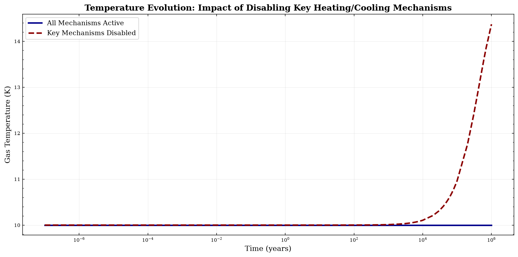
Step 7: Compare Results - Temperature Evolution#
Let’s compare the temperature evolution between the two models.
fig, ax = plt.subplots(figsize=(12, 6))

ax.plot(
    physics_full["Time"],
    physics_full["gasTemp"],
    label="All Mechanisms Active",
    linewidth=2.5,
    color="darkblue",
)
ax.plot(
    physics_limited["Time"],
    physics_limited["gasTemp"],
    label="Key Mechanisms Disabled",
    linewidth=2.5,
    color="darkred",
    linestyle="--",
)

ax.set_xlabel("Time (years)", fontsize=12)
ax.set_ylabel("Gas Temperature (K)", fontsize=12)
ax.set_xscale("log")
ax.set_title(
    "Temperature Evolution: Impact of Disabling Key Heating/Cooling Mechanisms",
    fontsize=14,
    fontweight="bold",
)
ax.legend(fontsize=11, loc="best")
ax.grid(True, alpha=0.3)

plt.tight_layout()
plt.show()

# Print summary statistics
print("TEMPERATURE COMPARISON")
print("=" * 70)
print(f"{'Model':<35} {'Initial (K)':<15} {'Final (K)':<15} {'Change (K)'}")
print("-" * 70)

T_full_initial = physics_full["gasTemp"].iloc[0]
T_full_final = physics_full["gasTemp"].iloc[-1]
T_limited_initial = physics_limited["gasTemp"].iloc[0]
T_limited_final = physics_limited["gasTemp"].iloc[-1]

print(
    f"{'All mechanisms':<35} {T_full_initial:<15.2f} {T_full_final:<15.2f} {T_full_final - T_full_initial:+.2f}"
)
print(
    f"{'Key mechanisms disabled':<35} {T_limited_initial:<15.2f} {T_limited_final:<15.2f} {T_limited_final - T_limited_initial:+.2f}"
)
print("-" * 70)
print(
    f"{'Difference':<35} {'':<15} {T_full_final - T_limited_final:<15.2f} {abs((T_full_final - T_limited_final) / T_full_final) * 100:.1f}%"
)
/tmp/ipykernel_3713/1143891968.py:30: UserWarning: The figure layout has changed to tight
  plt.tight_layout()
TEMPERATURE COMPARISON
======================================================================
Model                               Initial (K)     Final (K)       Change (K)
----------------------------------------------------------------------
All mechanisms                      10.00           10.00           +0.00
Key mechanisms disabled             10.00           14.37           +4.37
----------------------------------------------------------------------
Difference                                          -4.37           43.7%
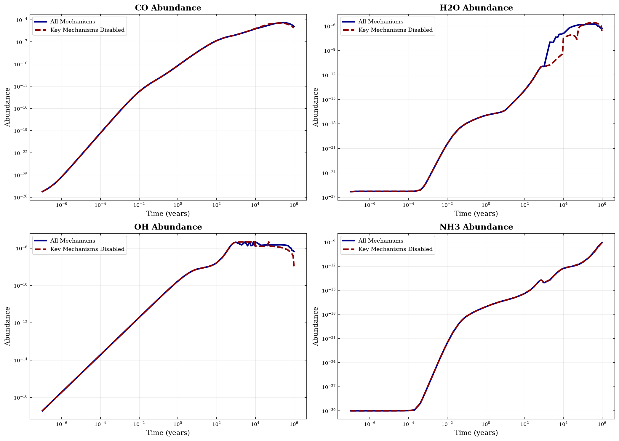
Step 8: Compare Results - Chemical Abundances#
Temperature changes affect chemistry. Let’s compare key species abundances between the two models.
# Compare abundances of key species
key_species = ["CO", "H2O", "OH", "NH3"]

fig, axes = plt.subplots(2, 2, figsize=(14, 10))
axes = axes.flatten()

for idx, species in enumerate(key_species):
    if species in abundances_full.columns and species in abundances_limited.columns:
        axes[idx].plot(
            physics_full["Time"],
            abundances_full[species],
            label="All Mechanisms",
            linewidth=2.5,
            color="darkblue",
        )
        axes[idx].plot(
            physics_full["Time"],
            abundances_limited[species],
            label="Key Mechanisms Disabled",
            linewidth=2.5,
            color="darkred",
            linestyle="--",
        )

        axes[idx].set_xlabel("Time (years)", fontsize=11)
        axes[idx].set_ylabel("Abundance", fontsize=11)
        axes[idx].set_xscale("log")
        axes[idx].set_yscale("log")
        axes[idx].set_title(f"{species} Abundance", fontsize=13, fontweight="bold")
        axes[idx].legend(fontsize=9)
        axes[idx].grid(True, alpha=0.3)

plt.tight_layout()
plt.show()

# Print final abundance comparison
print("\nFINAL ABUNDANCE COMPARISON")
print("=" * 70)
print(f"{'Species':<15} {'All Mechanisms':<20} {'Disabled':<20} {'% Difference'}")
print("-" * 70)

for species in key_species:
    if species in abundances_full.columns and species in abundances_limited.columns:
        abund_full = abundances_full[species].iloc[-1]
        abund_limited = abundances_limited[species].iloc[-1]

        if abund_full > 0:
            percent_diff = ((abund_limited - abund_full) / abund_full) * 100
        else:
            percent_diff = 0.0

        print(
            f"{species:<15} {abund_full:<20.2e} {abund_limited:<20.2e} {percent_diff:+.1f}%"
        )
/tmp/ipykernel_3713/3440187664.py:33: UserWarning: The figure layout has changed to tight
  plt.tight_layout()
FINAL ABUNDANCE COMPARISON
======================================================================
Species         All Mechanisms       Disabled             % Difference
----------------------------------------------------------------------
CO              1.24e-05             8.60e-06             -30.4%
H2O             5.22e-07             1.44e-07             -72.4%
OH              6.48e-09             1.05e-09             -83.8%
NH3             8.51e-10             1.07e-09             +26.3%
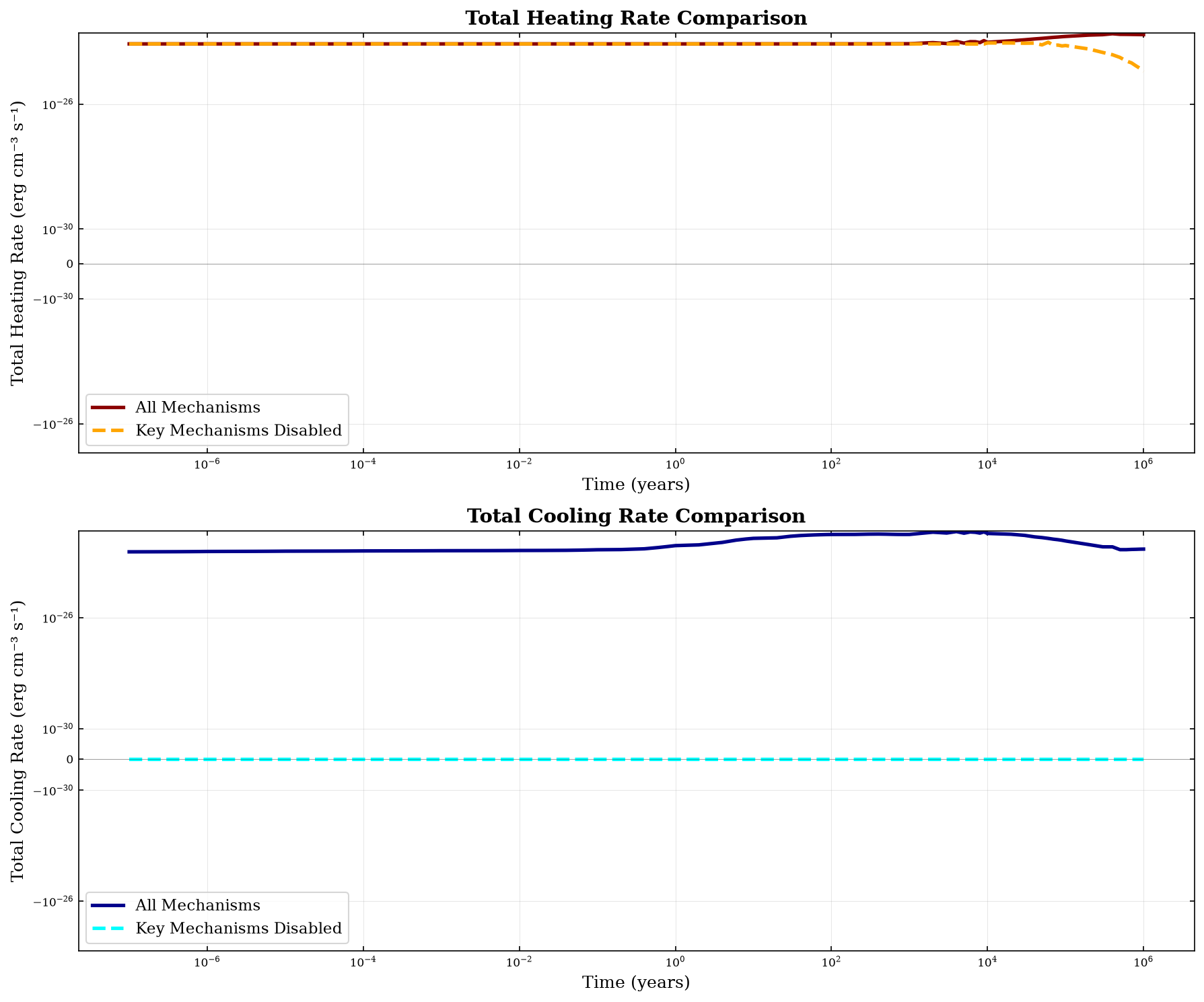
Step 9: Compare Heating and Cooling Rates#
Let’s visualize how the heating and cooling rates differ between the two models.
# Calculate total heating and cooling for each model
heating_cols_full = [col for col in heating_full.columns if col.endswith("Heating")]
cooling_cols_full = [col for col in heating_full.columns if col.endswith("Cooling")]

# Total heating and cooling rates over time
total_heating_full = heating_full[heating_cols_full].sum(axis=1)
total_cooling_full = heating_full[cooling_cols_full].sum(axis=1)

heating_cols_limited = [
    col for col in heating_limited.columns if col.endswith("Heating")
]
cooling_cols_limited = [
    col for col in heating_limited.columns if col.endswith("Cooling")
]

total_heating_limited = heating_limited[heating_cols_limited].sum(axis=1)
total_cooling_limited = heating_limited[cooling_cols_limited].sum(axis=1)

# Plot comparison
fig, axes = plt.subplots(2, 1, figsize=(12, 10))

# Total heating comparison
axes[0].plot(
    physics_full["Time"],
    total_heating_full,
    label="All Mechanisms",
    linewidth=2.5,
    color="darkred",
)
axes[0].plot(
    physics_limited["Time"],
    total_heating_limited,
    label="Key Mechanisms Disabled",
    linewidth=2.5,
    color="orange",
    linestyle="--",
)
axes[0].axhline(y=0, color="k", linestyle="-", linewidth=0.5, alpha=0.3)
axes[0].set_xlabel("Time (years)", fontsize=12)
axes[0].set_ylabel("Total Heating Rate (erg cm⁻³ s⁻¹)", fontsize=12)
axes[0].set_xscale("log")
axes[0].set_yscale("symlog", linthresh=1e-30)
axes[0].set_title("Total Heating Rate Comparison", fontsize=14, fontweight="bold")
axes[0].legend(fontsize=11)
axes[0].grid(True, alpha=0.3)

# Total cooling comparison
axes[1].plot(
    physics_full["Time"],
    total_cooling_full,
    label="All Mechanisms",
    linewidth=2.5,
    color="darkblue",
)
axes[1].plot(
    physics_limited["Time"],
    total_cooling_limited,
    label="Key Mechanisms Disabled",
    linewidth=2.5,
    color="cyan",
    linestyle="--",
)
axes[1].axhline(y=0, color="k", linestyle="-", linewidth=0.5, alpha=0.3)
axes[1].set_xlabel("Time (years)", fontsize=12)
axes[1].set_ylabel("Total Cooling Rate (erg cm⁻³ s⁻¹)", fontsize=12)
axes[1].set_xscale("log")
axes[1].set_yscale("symlog", linthresh=1e-30)
axes[1].set_title("Total Cooling Rate Comparison", fontsize=14, fontweight="bold")
axes[1].legend(fontsize=11)
axes[1].grid(True, alpha=0.3)

plt.tight_layout()
plt.show()

# Calculate net heating/cooling
net_full = total_heating_full + total_cooling_full
net_limited = total_heating_limited + total_cooling_limited

print("\nNET HEATING RATE AT FINAL TIME")
print("=" * 70)
print(f"All mechanisms:         {net_full.iloc[-1]:+.2e} erg cm⁻³ s⁻¹")
print(f"Mechanisms disabled:    {net_limited.iloc[-1]:+.2e} erg cm⁻³ s⁻¹")
print(
    f"Difference:             {net_full.iloc[-1] - net_limited.iloc[-1]:+.2e} erg cm⁻³ s⁻¹"
)
/tmp/ipykernel_3713/3480408715.py:72: UserWarning: The figure layout has changed to tight
  plt.tight_layout()
NET HEATING RATE AT FINAL TIME
======================================================================
All mechanisms:         +4.60e-24 erg cm⁻³ s⁻¹
Mechanisms disabled:    +1.08e-25 erg cm⁻³ s⁻¹
Difference:             +4.49e-24 erg cm⁻³ s⁻¹
Summary and Key Takeaways#
In this notebook, we demonstrated how to:
Run a baseline model with all heating and cooling mechanisms enabled
Analyze the results to identify which processes are most important
Disable specific mechanisms using the
HeatingSettingsclassCompare models to quantify the impact of individual processes
Important HeatingSettings Methods:#
get_heating_modules()- List all available heating mechanisms and their statusget_cooling_modules()- List all available cooling mechanisms and their statusset_heating_mechanism(mechanism, active)- Enable/disable a heating mechanismset_cooling_mechanism(mechanism, active)- Enable/disable a cooling mechanismreset()- Reset all mechanisms to defaults
Common Mechanism Constants:#
Heating:
settings.COSMIC_RAY- Cosmic ray heatingsettings.H2_FORMATION- H₂ formation heatingsettings.PHOTOELECTRIC- Photoelectric heating (various models)settings.PHOTODISSOCIATION- Photodissociation heatingsettings.TURBULENT- Turbulent heating
Cooling:
settings.CO_LINE_COOLING- CO line coolingsettings.H2_COLLISIONALLY_INDUCED- H₂ collisionally induced emissionsettings.ATOMIC_LINE_COOLING- Atomic fine structure coolingsettings.DUST_CONTINUUM- Dust continuum cooling
When to Use This:#
Physical insight: Understand which processes drive thermal evolution
Sensitivity analysis: Test model dependence on individual mechanisms
Simplified models: Disable processes not relevant to your environment
Debugging: Isolate problematic heating/cooling processes
Next Steps:#
Try different physical conditions (density, Av, radiation field)
Experiment with disabling different combinations of mechanisms
Compare to observations to validate dominant processes
See 5_heating_and_cooling.ipynb for basic heating/cooling usage