Heating and Cooling in UCLCHEM#
This notebook demonstheating how to use UCLCHEM with heating and cooling mechanisms enabled. UCLCHEM includes a comprehensive set of heating and cooling processes that can significantly affect the temperature evolution and chemistry in astrophysical environments.
Overview#
UCLCHEM can track gas temperature changes due to:
Heating processes:
Photoelectric heating from PAHs and dust grains
H₂ formation heating
H₂ photodissociation heating
Cosmic ray heating
Chemical reaction enthalpy (optional)
X-ray heating
Turbulent heating
And more…
Cooling processes:
Line cooling (CO, H₂O, OH, etc.)
Continuum cooling from dust
Atomic fine structure cooling (C⁺, O, etc.)
Recombination cooling
And more…
By default, heating is enabled (heatingFlag=True), but you can turn it off or customize which processes are included.
import matplotlib.pyplot as plt

import uclchem
Example 1: Basic Model with Heating Enabled#
Let’s start with a simple cloud model with heating and cooling enabled (the default behavior). We’ll model a molecular cloud core at constant density.
# Define parameters for a molecular cloud with heating enabled
param_dict_heating = {
    "initialDens": 1e4,  # Initial density (cm^-3)
    "initialTemp": 10.0,  # Initial temperature (K)
    "finalTime": 1.0e6,  # Final time (years)
    "baseAv": 10.0,  # Visual extinction
    "rout": 0.1,  # Outer radius (pc)
    "freefall": False,  # Keep constant density
    "heatingFlag": True,  # Enable heating (default)
}

# Run the model using the Cloud class
cloud = uclchem.model.Cloud(param_dict=param_dict_heating)

# Extract data from the model object
physics, abundances = cloud.get_dataframes(joined=False)
_, _, rate_constants = cloud.get_dataframes(joined=False, with_rate_constants=True)
_, _, heating = cloud.get_dataframes(joined=False, with_heating=True)
start_abund = cloud.next_starting_chemistry_array
flag = 0 if cloud.has_attr("_data") else -1

print(f"Model completed with flag: {flag}")
if flag < 0:
    print("Error: Model failed to complete")
else:
    print("Success! Model completed.")
    print(
        f"\nTemperature range: {physics['gasTemp'].min():.2f} - {physics['gasTemp'].max():.2f} K"
    )
    print(
        f"Density range: {physics['Density'].min():.2e} - {physics['Density'].max():.2e} cm^-3"
    )
Model completed with flag: -1
Error: Model failed to complete
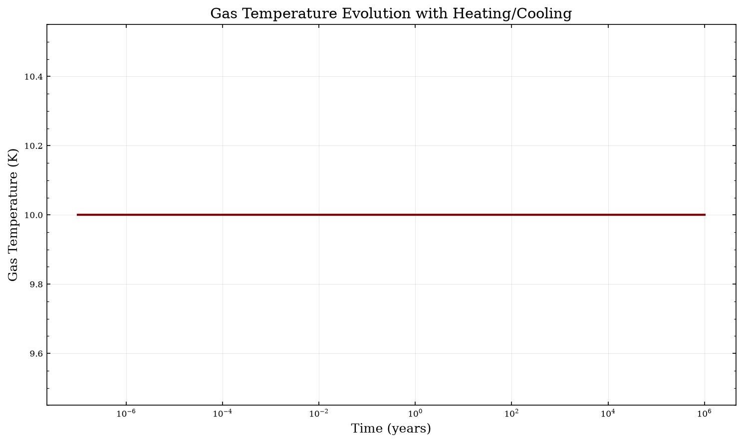
Visualizing Temperature Evolution#
The physics DataFrame contains physical properties including gas temperature. Let’s plot how temperature evolves over time.
# Plot temperature evolution
fig, ax = plt.subplots(figsize=(10, 6))
ax.plot(physics["Time"], physics["gasTemp"], linewidth=2, color="darkred")
ax.set_xlabel("Time (years)", fontsize=12)
ax.set_ylabel("Gas Temperature (K)", fontsize=12)
ax.set_xscale("log")
ax.set_title("Gas Temperature Evolution with Heating/Cooling", fontsize=14)
ax.grid(True, alpha=0.3)
plt.tight_layout()
plt.show()
/tmp/ipykernel_3657/1204520022.py:9: UserWarning: The figure layout has changed to tight
  plt.tight_layout()
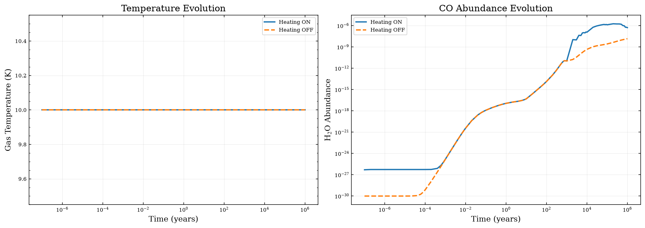
Example 2: Comparing Heating On vs Off#
To see the impact of heating/cooling processes, let’s run two models side by side: one with heating enabled and one without.
# Model WITHOUT heating
param_dict_no_heating = param_dict_heating.copy()
param_dict_no_heating["heatingFlag"] = False

cloud_no_heat = uclchem.model.Cloud(param_dict=param_dict_no_heating)

# Extract data
physics_no_heat, abundances_no_heat = cloud_no_heat.get_dataframes(joined=False)
_, _, rate_constants_no_heat = cloud_no_heat.get_dataframes(joined=False, with_rate_constants=True)
_, _, heating_no_heat = cloud_no_heat.get_dataframes(joined=False, with_heating=True)
flag_no_heat = 0 if cloud_no_heat.has_attr("_data") else -1

print(f"No heating model completed with flag: {flag_no_heat}")

# Compare the two runs
fig, axes = plt.subplots(1, 2, figsize=(14, 5))

# Temperature comparison
axes[0].plot(physics["Time"], physics["gasTemp"], label="Heating ON", linewidth=2)
axes[0].plot(
    physics_no_heat["Time"],
    physics_no_heat["gasTemp"],
    label="Heating OFF",
    linewidth=2,
    linestyle="--",
)
axes[0].set_xlabel("Time (years)", fontsize=12)
axes[0].set_ylabel("Gas Temperature (K)", fontsize=12)
axes[0].set_xscale("log")
axes[0].set_title("Temperature Evolution", fontsize=14)
axes[0].legend()
axes[0].grid(True, alpha=0.3)

# Compare a key chemical species (CO)
axes[1].plot(physics["Time"], abundances["H2O"], label="Heating ON", linewidth=2)
axes[1].plot(
    physics_no_heat["Time"],
    abundances_no_heat["H2O"],
    label="Heating OFF",
    linewidth=2,
    linestyle="--",
)
axes[1].set_xlabel("Time (years)", fontsize=12)
axes[1].set_ylabel("H$_2$O Abundance", fontsize=12)
axes[1].set_xscale("log")
axes[1].set_yscale("log")
axes[1].set_title("CO Abundance Evolution", fontsize=14)
axes[1].legend()
axes[1].grid(True, alpha=0.3)

plt.tight_layout()
plt.show()

print("\nFinal temperatures:")
print(f"  With heating: {physics['gasTemp'].iloc[-1]:.2f} K")
print(f"  Without heating: {physics_no_heat['gasTemp'].iloc[-1]:.2f} K")
No heating model completed with flag: -1

Final temperatures:
  With heating: 10.00 K
  Without heating: 10.00 K
/tmp/ipykernel_3657/477657872.py:51: UserWarning: The figure layout has changed to tight
  plt.tight_layout()
Example 3: Accessing Heating and Cooling Rates#
UCLCHEM can return detailed heating and cooling rates when you use return_dataframe=True with the rates arrays. The heating DataFrame includes individual contributions from each heating and cooling process.
# The heating DataFrame contains heating and cooling information
print("Available heating/cooling columns:")
print(heating.columns.tolist()[:20], "...")  # Show first 20 columns

# Extract heating and cooling columns
heating_cols = [
    col for col in heating.columns if "heating" in col.lower() and col != "Time"
]
cooling_cols = [col for col in heating.columns if "cooling" in col.lower()]

print(f"\nFound {len(heating_cols)} heating processes")
print(f"Found {len(cooling_cols)} cooling processes")

# Show the heating processes
print("\nHeating processes:")
for col in heating_cols[:10]:  # Show first 10
    print(f"  - {col}")
Available heating/cooling columns:
['Point', 'Time', 'AtomicLineEmission Cooling', 'H2CollisionallyInduced Cooling', 'Compton Cooling', 'ContinuumEmission Cooling', 'MolecularLine Cooling', 'H Line Cooling', 'C+ Line Cooling', 'O Line Cooling', 'C Line Cooling', 'CO Line Cooling', 'p-H2 Line Cooling', 'o-H2 Line Cooling', 'PhotoelectricBakes Heating', 'PhotoelectricWeingartner Heating', 'H2Formation Heating', 'H2Photodissociation Heating', 'H2FUVPumping Heating', 'CarbonIonization Heating'] ...

Found 10 heating processes
Found 12 cooling processes

Heating processes:
  - PhotoelectricBakes Heating
  - PhotoelectricWeingartner Heating
  - H2Formation Heating
  - H2Photodissociation Heating
  - H2FUVPumping Heating
  - CarbonIonization Heating
  - CosmicRay Heating
  - Turbulent Heating
  - GasGrainCollisions Heating
  - Chemical Heating
heating
| Point | Time | AtomicLineEmission Cooling | H2CollisionallyInduced Cooling | Compton Cooling | ContinuumEmission Cooling | MolecularLine Cooling | H Line Cooling | C+ Line Cooling | O Line Cooling | ... | PhotoelectricBakes Heating | PhotoelectricWeingartner Heating | H2Formation Heating | H2Photodissociation Heating | H2FUVPumping Heating | CarbonIonization Heating | CosmicRay Heating | Turbulent Heating | GasGrainCollisions Heating | Chemical Heating | |
|---|---|---|---|---|---|---|---|---|---|---|---|---|---|---|---|---|---|---|---|---|---|
| 0 | 1 | 1.000000e-07 | 0.0 | 0.0 | 7.495208e-35 | 2.994978e-63 | 1.177133e-24 | 0.000000e+00 | 3.325834e-25 | 8.444844e-25 | ... | -1.101706e-34 | 0.0 | 2.546569e-40 | 5.689194e-43 | 9.946882e-50 | 4.516163e-48 | 8.339649e-25 | 7.007000e-40 | 3.974870e-28 | 0.0 |
| 1 | 1 | 2.000000e-07 | 0.0 | 0.0 | 7.495208e-35 | 2.994978e-63 | 1.183107e-24 | 0.000000e+00 | 3.314459e-25 | 8.515956e-25 | ... | -1.097683e-34 | 0.0 | 8.488072e-31 | 5.649444e-43 | 9.877383e-50 | 4.490500e-48 | 8.339649e-25 | 7.007000e-40 | 3.974870e-28 | 0.0 |
| 2 | 1 | 4.000000e-07 | 0.0 | 0.0 | 7.495208e-35 | 2.994978e-63 | 1.190512e-24 | 0.000000e+00 | 3.312229e-25 | 8.592256e-25 | ... | -1.097683e-34 | 0.0 | 9.725541e-31 | 5.649444e-43 | 9.877383e-50 | 4.497471e-48 | 8.339649e-25 | 7.007000e-40 | 3.974870e-28 | 0.0 |
| 3 | 1 | 6.000000e-07 | 0.0 | 0.0 | 7.495208e-35 | 2.994978e-63 | 1.197835e-24 | 0.000000e+00 | 3.311603e-25 | 8.666113e-25 | ... | -1.097683e-34 | 0.0 | 9.808846e-31 | 5.649444e-43 | 9.877383e-50 | 4.511414e-48 | 8.339649e-25 | 7.007000e-40 | 3.974870e-28 | 0.0 |
| 4 | 1 | 8.000000e-07 | 0.0 | 0.0 | 7.495208e-35 | 2.994978e-63 | 1.204947e-24 | 0.000000e+00 | 3.311428e-25 | 8.737416e-25 | ... | -1.097683e-34 | 0.0 | 9.817773e-31 | 5.649444e-43 | 9.877383e-50 | 4.525357e-48 | 8.339649e-25 | 7.007000e-40 | 3.974870e-28 | 0.0 |
| ... | ... | ... | ... | ... | ... | ... | ... | ... | ... | ... | ... | ... | ... | ... | ... | ... | ... | ... | ... | ... | ... |
| 81 | 1 | 6.000000e+05 | 0.0 | 0.0 | 9.925196e-37 | 2.658868e-64 | 1.409810e-24 | 2.386645e-25 | 3.344522e-29 | 1.510227e-25 | ... | -6.298685e-36 | 0.0 | 5.038912e-28 | 6.272619e-43 | 9.441355e-50 | 3.550028e-43 | 1.028097e-24 | 7.007000e-40 | 6.540557e-25 | 0.0 |
| 82 | 1 | 7.000000e+05 | 0.0 | 0.0 | 1.116521e-36 | 3.368501e-64 | 1.437747e-24 | 2.458275e-25 | 3.028306e-29 | 1.074064e-25 | ... | -7.408213e-36 | 0.0 | 4.632120e-28 | 6.338668e-43 | 1.007680e-49 | 2.801883e-43 | 1.049862e-24 | 7.007000e-40 | 6.243741e-25 | 0.0 |
| 83 | 1 | 8.000000e+05 | 0.0 | 0.0 | 1.326426e-36 | 3.955641e-64 | 1.450765e-24 | 2.508146e-25 | 3.365368e-29 | 8.204044e-26 | ... | -8.552798e-36 | 0.0 | 4.349505e-28 | 6.386348e-43 | 1.054610e-49 | 2.243279e-43 | 1.065716e-24 | 7.007000e-40 | 6.011325e-25 | 0.0 |
| 84 | 1 | 9.000000e+05 | 0.0 | 0.0 | 1.443596e-36 | 4.674011e-64 | 1.468489e-24 | 2.561014e-25 | 2.905628e-29 | 5.993557e-26 | ... | -9.607630e-36 | 0.0 | 4.036668e-28 | 6.441090e-43 | 1.108305e-49 | 1.855935e-43 | 1.084065e-24 | 7.007000e-40 | 5.741312e-25 | 0.0 |
| 85 | 1 | 1.000000e+06 | 0.0 | 0.0 | 1.551650e-36 | 5.514994e-64 | 1.476265e-24 | 2.614532e-25 | 2.531119e-29 | 4.069889e-26 | ... | -1.074130e-35 | 0.0 | 3.701012e-28 | 6.502444e-43 | 1.167956e-49 | 1.486357e-43 | 1.104815e-24 | 7.007000e-40 | 5.442690e-25 | 0.0 |
86 rows × 24 columns
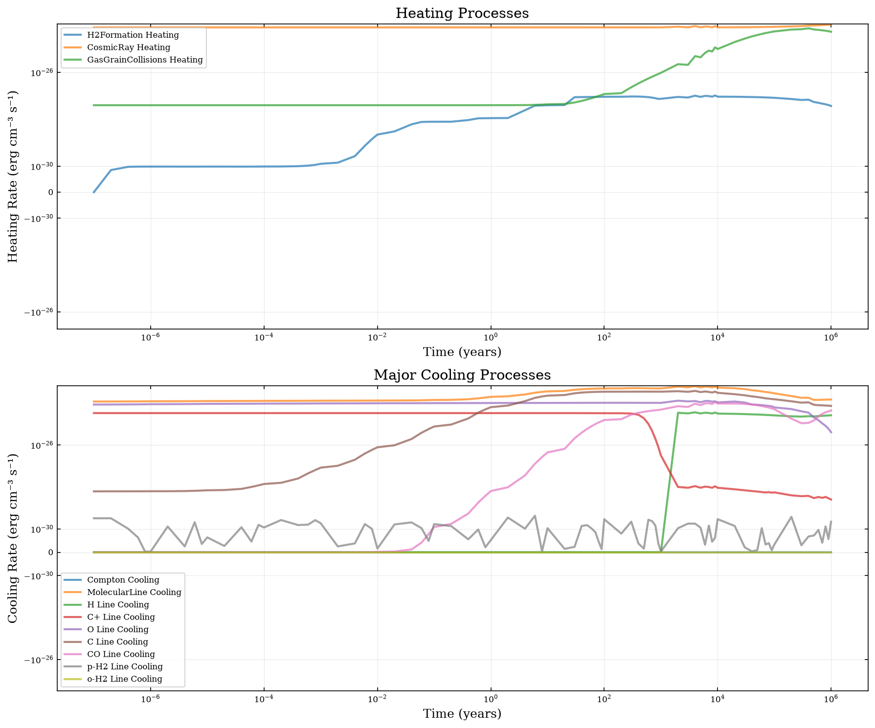
Plotting Individual Heating and Cooling Contributions#
Let’s visualize the dominant heating and cooling processes over time.
fig, axes = plt.subplots(2, 1, figsize=(12, 10))

# Plot heating processes
time = physics["Time"]
for col in heating_cols:
    # Only plot processes with significant contribution
    max_val = heating[col].abs().max()
    if max_val > 1e-30:  # Filter out negligible contributions
        label = col.replace("_heating", "").replace("_", " ")
        axes[0].plot(time, heating[col], label=label, linewidth=2, alpha=0.7)

axes[0].set_xlabel("Time (years)", fontsize=12)
axes[0].set_ylabel("Heating Rate (erg cm⁻³ s⁻¹)", fontsize=12)
axes[0].set_xscale("log")
axes[0].set_yscale("symlog", linthresh=1e-30)
axes[0].set_title("Heating Processes", fontsize=14)
axes[0].legend(fontsize=8, loc="best")
axes[0].grid(True, alpha=0.3)

# Plot cooling processes (select major ones to avoid cluttering)
for col in cooling_cols:
    max_val = heating[col].abs().max()
    if max_val > 1e-40:
        label = col.replace("_cooling", "").replace("_", " ")
        axes[1].plot(time, heating[col], label=label, linewidth=2, alpha=0.7)

axes[1].set_xlabel("Time (years)", fontsize=12)
axes[1].set_ylabel("Cooling Rate (erg cm⁻³ s⁻¹)", fontsize=12)
axes[1].set_xscale("log")
axes[1].set_yscale("symlog", linthresh=1e-30)
axes[1].set_title("Major Cooling Processes", fontsize=14)
axes[1].legend(fontsize=8, loc="best")
axes[1].grid(True, alpha=0.3)

plt.tight_layout()
plt.show()
/tmp/ipykernel_3657/2891720901.py:35: UserWarning: The figure layout has changed to tight
  plt.tight_layout()
Example 4: Writing Heating Rates to a File#
You can also save heating and cooling rates directly to a file during the model run using the heatingFile parameter. This requires not running any other cells to memory before!
# You can uncomment the cel below to run a model to disk.

# # Run model with heating file output
# param_dict_with_file = param_dict_heating.copy()
# param_dict_with_file["outputFile"] = "../examples/test-output/heating_demo.dat"
# param_dict_with_file["heatingFile"] = "../examples/test-output/heating_rates.dat"


# result = uclchem.model.cloud(
#     param_dict=param_dict_with_file, out_species=["CO", "H2O", "OH"]
# )

# print(f"Model completed with flag: {result[0]}")
# print(f"Final CO abundance: {result[1]:.2e}")
# print(f"Final H2O abundance: {result[2]:.2e}")
# print(f"Final OH abundance: {result[3]:.2e}")

# # Read the heating file
# if os.path.exists("../examples/test-output/heating_rates.dat"):
#     print("\nHeating rates file created successfully!")
#     heating_df = pd.read_csv("../examples/test-output/heating_rates.dat")
#     print(f"File contains {len(heating_df)} time steps")
#     print(f"Columns: {heating_df.columns.tolist()[:10]}...")  # Show first 10 columns
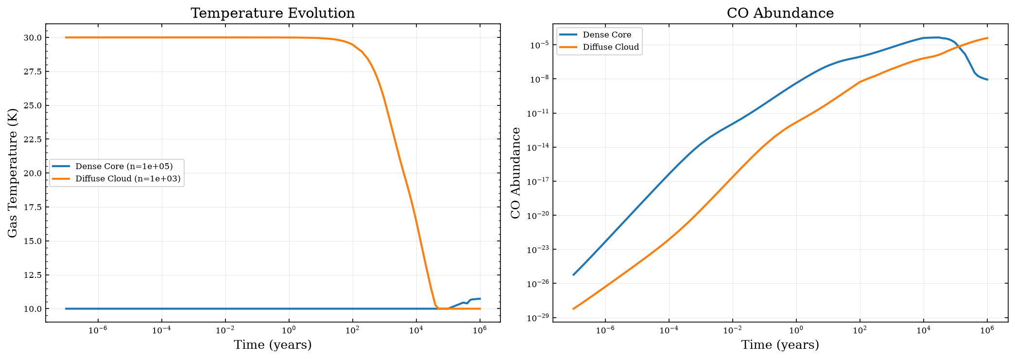
Example 5: Different Physical Conditions#
Let’s explore how heating and cooling behave under different physical conditions. We’ll compare a dense, cold core with a less dense, warmer environment.
# Dense, cold core (like Example 1)
param_cold_core = {
    "initialDens": 1e5,
    "initialTemp": 10.0,
    "finalTime": 1.0e6,
    "baseAv": 20.0,
    "rout": 0.05,
    "freefall": False,
    "heatingFlag": True,
}

# Less dense, warmer cloud
param_warm_cloud = {
    "initialDens": 1e3,
    "initialTemp": 30.0,
    "finalTime": 1.0e6,
    "baseAv": 5.0,
    "rout": 0.5,
    "freefall": False,
    "heatingFlag": True,
}

# Run both models
print("Running cold core model...")
cloud_cold = uclchem.model.Cloud(param_dict=param_cold_core)
phys_cold, abund_cold = cloud_cold.get_dataframes(joined=False)
_, _, rate_constants_cold = cloud_cold.get_dataframes(joined=False, with_rate_constants=True)
_, _, heating_cold = cloud_cold.get_dataframes(joined=False, with_heating=True)
flag_cold = 0 if cloud_cold.has_attr("_data") else -1

print("Running warm cloud model...")
cloud_warm = uclchem.model.Cloud(param_dict=param_warm_cloud)
phys_warm, abund_warm = cloud_warm.get_dataframes(joined=False)
_, _, rate_constants_warm = cloud_warm.get_dataframes(joined=False, with_rate_constants=True)
_, _, heating_warm = cloud_warm.get_dataframes(joined=False, with_heating=True)
flag_warm = 0 if cloud_warm.has_attr("_data") else -1

print(f"\nCold core flag: {flag_cold}, Warm cloud flag: {flag_warm}")

# Compare temperature evolution
fig, axes = plt.subplots(1, 2, figsize=(14, 5))

axes[0].plot(
    phys_cold["Time"],
    phys_cold["gasTemp"],
    label=f"Dense Core (n={param_cold_core['initialDens']:.0e})",
    linewidth=2,
)
axes[0].plot(
    phys_warm["Time"],
    phys_warm["gasTemp"],
    label=f"Diffuse Cloud (n={param_warm_cloud['initialDens']:.0e})",
    linewidth=2,
)
axes[0].set_xlabel("Time (years)", fontsize=12)
axes[0].set_ylabel("Gas Temperature (K)", fontsize=12)
axes[0].set_xscale("log")
axes[0].set_title("Temperature Evolution", fontsize=14)
axes[0].legend()
axes[0].grid(True, alpha=0.3)

# Compare CO abundance
axes[1].plot(phys_cold["Time"], abund_cold["CO"], label="Dense Core", linewidth=2)
axes[1].plot(phys_warm["Time"], abund_warm["CO"], label="Diffuse Cloud", linewidth=2)
axes[1].set_xlabel("Time (years)", fontsize=12)
axes[1].set_ylabel("CO Abundance", fontsize=12)
axes[1].set_xscale("log")
axes[1].set_yscale("log")
axes[1].set_title("CO Abundance", fontsize=14)
axes[1].legend()
axes[1].grid(True, alpha=0.3)

plt.tight_layout()
plt.show()

print("\nFinal temperatures:")
print(f"  Cold core: {phys_cold['gasTemp'].iloc[-1]:.2f} K")
print(f"  Warm cloud: {phys_warm['gasTemp'].iloc[-1]:.2f} K")
Running cold core model...
Running warm cloud model...
[last_model]  At T(=R1) and step size H(=R2), the
[last_model]  corrector convergence failed repeatedly
[last_model]  or with ABS(H) = HMIN.
[last_model] In the above message, R1 =   0.1795551817850D+10   R2 =   0.6154874025949D+02
[last_model]  ISTATE -5 - shortening step at time   50.000000000000000      years

Cold core flag: -1, Warm cloud flag: -1

Final temperatures:
  Cold core: 10.73 K
  Warm cloud: 10.00 K
/tmp/ipykernel_3657/10617990.py:73: UserWarning: The figure layout has changed to tight
  plt.tight_layout()
Summary of Key Heating and Cooling Processes#
UCLCHEM includes the following heating and cooling mechanisms:
Major Heating Processes:#
Photoelectric heating - from PAHs and dust grains (Bakes & Tielens 1994)
H₂ formation heating - energy released during H₂ formation on grains
H₂ photodissociation heating - kinetic energy from photodissociation
Cosmic ray heating - direct and indirect (via ionization)
Chemical reaction enthalpy - exothermic reactions (optional, requires network configuration)
X-ray heating - in environments with X-ray sources
Turbulent heating - dissipation of turbulent energy
Viscous heating - for shock models
Major Cooling Processes:#
Molecular line cooling - CO, H₂O, OH, and other molecules
Atomic fine structure cooling - C⁺, O, C, etc.
Dust continuum cooling - gas-grain collisional cooling
H₂ line cooling - rovibrational transitions
Recombination cooling - electronic to kinetic energy
Ly-α cooling - Lyman-alpha photon emission
Key Parameters:#
heatingFlag: Enable/disable all heating processes (default:True)heatingFile: Path to write detailed heating/cooling ratesinitialTemp: Starting gas temperaturebaseAv: Visual extinction (affects radiation field attenuation)zeta: Cosmic ray ionization rate
For a complete list of processes and their equations, see the HEATING_COOLING_SUMMARY.md documentation file.
Advanced: Chemical Reaction Enthalpy#
UCLCHEM can optionally include the enthalpy changes from chemical reactions as a heating/cooling source. This requires configuring the chemical network at build time using MakeRates.
Note: This feature requires rebuilding UCLCHEM with specific settings in the user_settings.yaml file. The main settings are:
add_delta_enthalpy: Can beFalse,GAS, orALLFalse: No reaction enthalpy (default)GAS: Include enthalpy from gas-phase reactions onlyALL: Include enthalpy from all reactions (gas + surface)
To enable reaction enthalpy:
# In Makerates/user_settings.yaml
add_delta_enthalpy: GAS
Then rebuild:
cd Makerates
python MakeRates.py
cd ..
pip install .
For more details, see the heating_cooling_benchmarks/ directory which contains examples with different enthalpy configurations.
Tips for Using Heating and Cooling#
Always check convergence: Use
return_dataframe=Trueand inspect temperature evolution to ensure physical resultsMonitor element conservation: Use
uclchem.analysis.check_element_conservation()to verify model accuracySave heating rates for analysis: Use
heatingFileparameter to save detailed heating/cooling contributionsChoose appropriate tolerances: If you see unphysical temperature spikes, try adjusting
reltolandabstolparametersConsider your environment: Different astrophysical environments have different dominant heating/cooling processes:
Dense cores: Line cooling (CO, H₂O) dominates
Diffuse clouds: Photoelectric heating and fine-structure cooling
Shock regions: Viscous/turbulent heating important
PDRs: Strong FUV field means photoelectric heating dominates
Radiation field matters: The
baseAvparameter controls UV attenuation, which significantly affects photoelectric heating and photodissociation rates
Next Steps#
Check out 7_heating_cooling_settings.ipynb for more advanced configuration options
See
HEATING_COOLING_SUMMARY.mdfor detailed equations and referencesExplore the
heating_cooling_benchmarks/directory for systematic comparisons