Core Physics

Each of the other physics doc pages details the specifics of a particular physics model. This one gives a general overview of the physics in UCLCHEM, including the core physics routines that are called for all models.

Model dimensions

Whilst it is most often used to model a single point, UCLCHEM is a 1D model. For most models, you provide the size of some cloud of gas (rout) and the number of positions along a 1D cut through this cloud you'd like to model (points). UCLCHEM then divides the cloud up into the required number of equally sized segments and then models a point at the inner edge of each segment. In the image below, the user has specified that they would like to model six points between some rin and rout. The cloud has been split into six segments and the dots indicate the exact position at which

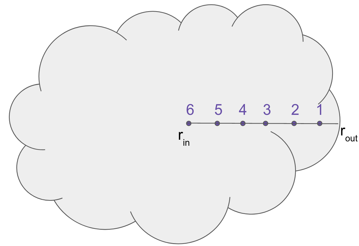
The reason we have to specify the exact position of the "point" at which UCLCHEM evaluates the abundances is that it affects the column densities. We start our calculation at the edge (hence point 1 is closest to rout) and use the width of a single segment to calculate the column densities of H2, CO, and C as well as the total column density. This affects the photo-chemistry through UV attenuation and self-shielding. However, it is unlikely a user will model enough points to properly follow the UV chemistry in the low A$_V$ parts of the cloud, especially since the time dependent nature of the code means it could take some time. If a full 1D calculation becomes really important to you, you may wish to consider a more purpose built PDR solver such as 3D-PDR.

A a result, we typically use UCLCHEM to model the cloud as a single point. Once we are far enough into the cloud that the A$_V$ is very high, the entire cloud tends to become homogenous in 1D models. Effectively, you can model the entire cloud with Av greater than about 5 as a single point and assume those abundances hold for the entire UV shielded region of the cloud. However, our 1D set up is useful for things like hot cores where the temperature and chemistry is really dominated by the central heating source, for which we treat the radial dependence quite well. You can then get a radial view of the chemistry with just a few points.

Core Physics Processes

Freefall

Many, but not all, models allow you to allow the gas to increase in density as if the gas begins to collapse under freefall from being stationary at the intial density. You turn this on with the freefall toggle and the analytical equation for this is

$$\frac{dn}{dt} = b_c \left(\frac{n^4}{n_0}\right)^{\frac{1}{3}}\left[24\pi Gm_Hn_0\left(\left(\frac{n}{n_0}\right)^{\frac{1}{3}}-1\right)\right]^{\frac{1}{2}}$$

this is the rate of change of the number density of H nuclei (that is our density unit) which is passed to the integrator to be intregrated over time along with the abundances. $b_c$ is freefallFactor in the parameters, a factor used to slow the collapse. $n_0$ is the code's initialDens parameter. We stop this collapse at finalDens even if the model continues.

Column density

We calculate the column density for a single point model or for the position closest to the cloud edge in 1D models, by dividing the total size of the cloud by the number of points and multiplying by density.

$$N_{Tot} = \frac{r_{cloud}}{N_{points}} n(r)$$

For points further in, we simply do the same calculation but then add the column density of the previous point. If we work in from the edge (point 1) to the centre (point N), then we get the cumulative column density. A similar process is followed for the column densities of CO, H2 and C.

We can then calculate the Av,

$$Av = Av_0 + \frac{N_{Tot}}{1.6 \times 10^{21} cm^{-2}}$$

where $Av_0$ is the code's baseAv parameter.