Running Your First Models with Objects

In this notebook, we demonstrate the basic use of UCLCHEM’s python module by running a simple model and then using the analysis functions to examine the output. Otherwise, it is identical to notebook 3.

import uclchem

A Simple Cloud

UCLCHEM’s Cloud class, models a spherical cloud of isothermal gas. We can keep a constant density or have it increase over time following a freefall equation. This model is generally useful whenever you want to model a homogeneous cloud of gas under constant conditions. For example, in the inner parts of a molecular cloud where Av \(\gtrsim\) 10 there are very few depth dependent processes. You may wish to model the whole of this UV shielded portion of the cloud with a single Cloud model.

Due to the large number of parameters in a chemical model and the way fortran and python interaction, we find it is easiest to do parameter input through python dictionaries. In this block, we define param_dict which contains the parameters we wish to modify for this run. Every uclchem.model class accepts a dictionary as an optional argument. Every parameter has a default value which is overridden if that parameter is specified in this dictionary. You can find a complete list of modifiable parameters and their default values in our parameter docs.

# set a parameter dictionary for phase 1 collapse model
out_species = ["SO", "CO"]
param_dict = {
    "endAtFinalDensity": False,  # stop at finalTime
    "freefall": False,  # don't increase density in freefall
    "initialDens": 1e4,  # starting density
    "initialTemp": 10.0,  # temperature of gas
    "finalTime": 1.0e6,  # final time
    "rout": 0.1,  # radius of cloud in pc
    "baseAv": 1.0,  # visual extinction at cloud edge.
}
cloud = uclchem.model.Cloud(param_dict=param_dict, out_species=out_species)
cloud.check_error()

Model ran successfully.

Checking the output

The code above produced the object cloud which holds the variables associated to the model that UCLCHEM calculated. Calling cloud.success_flag would exposes the variable success_flag which will be 0 if the model was run successfully, and negative if not. You can check an error value by calling cloud.check_error() to get a more detailed error message.

Additionally, the cloud object holds the physical parameters and chemical abundance arrays calculated by UCLCHEM. These are stored in cloud.physics_array and cloud.chemical_abun_array respectively. If we wish to see just the abundances of the final time step, we can get that array with cloud.next_starting_chemistry, bearing in mind that the variable cloud.starting_chemistry contains the array of abundances that the model started with, if it was provided to the object.

If abundSaveFile was added to the param_dict, then the final abundances of all species would be written to the file listed in abundSaveFile. If outputFile is added, then all abundances and physical parameters for all time steps will be written to the file outputFile.

The UCLCHEM model classes have methods to reformat the output arrays into pandas dataframes, as well as having the option to read previously run model output files. To retrieve a pandas dataframe of a model we can call cloud.get_dataframes(point = 0) where the point optional input allows us to choose which point we wish to retrieve the dataframe for, if we ran a multipoint model. This method defaults the point value to 0 to retrieve the central point.

cloud.get_dataframes().head()

	Time	Density	gasTemp	dustTemp	Av	radfield	zeta	dstep	H	H+	...	@OCS	@C4N	@SIC3	@SO2	@S2	@HS2	@H2S2	E-	BULK	SURFACE
0	1.000000e-07	10000.0	10.0	10.0	2.92875	1.0	2.910002	1.0	0.5	9.674388e-18	...	1.000000e-30	1.000000e-30	1.000000e-30	1.000000e-30	1.000000e-30	1.000000e-30	1.000000e-30	0.000182	5.613460e-20	7.478491e-13
1	1.000000e-06	10000.0	10.0	10.0	2.92875	1.0	2.910002	1.0	0.5	2.630577e-16	...	1.000001e-30	1.000001e-30	1.000001e-30	1.000001e-30	1.000001e-30	1.000001e-30	1.000001e-30	0.000182	5.546864e-18	7.434018e-12
2	1.000000e-05	10000.0	10.0	10.0	2.92875	1.0	2.910002	1.0	0.5	2.798139e-15	...	1.000015e-30	1.000015e-30	1.000015e-30	1.000015e-30	1.000015e-30	1.000015e-30	1.000015e-30	0.000182	5.538897e-16	7.428646e-11
3	1.000000e-04	10000.0	10.0	10.0	2.92875	1.0	2.910002	1.0	0.5	2.827256e-14	...	1.000147e-30	1.000147e-30	1.000147e-30	1.000147e-30	1.000147e-30	1.000147e-30	1.000148e-30	0.000182	5.418362e-14	7.347047e-10
4	1.000000e-03	10000.0	10.0	10.0	2.92875	1.0	2.910002	1.0	0.5	2.943250e-13	...	1.001110e-30	1.001110e-30	1.001110e-30	1.001110e-30	1.000926e-30	1.001081e-30	1.001335e-30	0.000182	3.072463e-12	5.530733e-09

5 rows × 343 columns

We can also test whether the model run went well by checking for element conservation. We do this because integrator errors often show up as a failure to conserve elemental abundances.

We can use cloud.check_conservation(element_list=["H", "N", "C", "O", "S"]) to test whether we conserve elements in this run. This method prints the conservation results of elements listed in the argument element_list as a percentage of the original abundance by default. In an ideal case, these values are 0% indicating the total abundance at the end of the model is exactly the same as the total at the start.

Changes of less than 1% are fine for many cases but if they are too high, you could consider changing the reltol and abstol parameters that control the integrator accuracy. They are error tolerance, so smaller values lead to smaller errors and (usually) longer integration times. The default values were chosen by running a large grid of models and choosing the tolerances with the lowest average run time from those that conserved elements well and rarely failed. Despite this, there are no one-size-fits-all perfect tolerances, and you may run into issues with different networks or models.

cloud.check_conservation(element_list=["H", "N", "C", "O", "S"])

Element conservation report
{'H': '0.000%', 'N': '0.000%', 'C': '0.000%', 'O': '0.000%', 'S': '0.000%'}

Plotting Results

Finally, you will want to plot your results. This can be done with any plotting library but UCLCHEM does provide a few functions to make quick plots. Note the use of $ symbols in the species list below, this gets the total ice abundance of a species. For two phase models, this is just the surface abudance but for three phase it is the sum of surface and bulk.

fig, ax = cloud.create_abundance_plot(
    species=["H", "H2", "$H", "$H2", "H2O", "$H2O", "CO", "$CO", "$CH3OH", "CH3OH"],
    figsize=(10, 7),
)
ax = ax.set(xscale="log", ylim=(1e-15, 1), xlim=(1e3, 1e6))

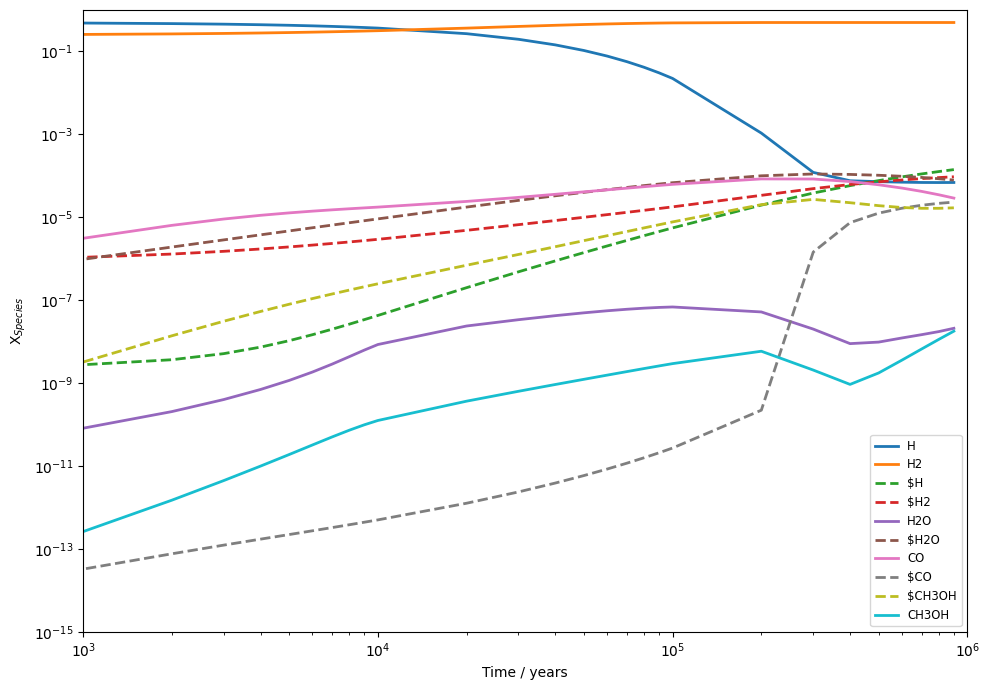
and that’s it! You’ve run your first UCLCHEM model, checked that the element conservation is correct, and plotted the abundances.